panda库使用方法
初始化
import pandas as pd
import numpy as np
df = pd.DataFrame({'A': 'foo bar foo bar foo bar foo foo'.split(),
                   'B': 'one one two three two two one three'.split(),
                   'C': np.arange(8), 'D': np.arange(8) * 2})
print(df)

df = pd.DataFrame({'Time':[1581350400,1581436800,1581523200,1581609600,1581696000],'Close':[9993.93,10251.64,10253.8,10314.59,10162.1]})


df = pd.DataFrame({'para':[1,2,3,4,5,6,7],'perf':[5,6,8,8,8,7,6]})

df = pd.DataFrame(index=[x for x in range(2009, 2019)])
sharp_list = []
# ……
df[stock] = sharp_list

# 超过55日高点
high_55day = max(dw.iloc[-56:-1].High.values)

# intialise data of dict.
data = {'Name':['Tom', 'nick', 'krish', 'jack'],
        'Age':[20, 21, 19, 18]}

# Create DataFrame
df = pd.DataFrame(data)

# intialise data of dict list
a=[{'年化收益/回撤比': [0], '累积净值': [1], '年化收益': [0], 'sharpe': [0]},{'年化收益/回撤比': [0], '累积净值': [1], '年化收益': [0], 'sharpe': [0]}]
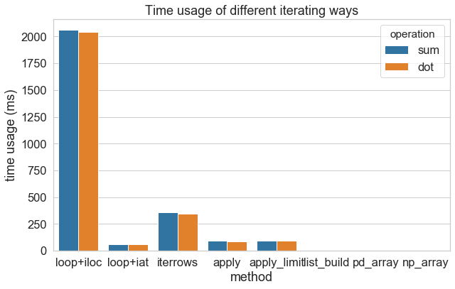
遍历
for循环+iloc < pd.iterrows < for循环+at < pd.apply pd列表构造 = np列表构造
# python 循環 + iat 定位
def method1_times(DF):
    for i in range(len(DF)):
        DF.iat[i,4] = DF.iat[i,0] * DF.iat[i,1]

# pandas.DataFrame.iterrows() 迭代器
def method2_times(DF):
    for index, rows in DF.iterrows():
        rows['eee'] = rows['aaa'] * rows['bbb']

# pandas.DataFrame.apply 迭代
def method3_times(DF):
    DF['eee'] = DF.apply(lambda x: x.aaa * x.bbb, axis=1)

# pandas.DataFrame.apply 迭代 + 只讀兩列
def method4_times(DF):
    DF['eee'] = DF[['aaa','bbb']].apply(lambda x: x.aaa * x.bbb, axis=1)
索引
dw = DataFrame(columns=['Time','Open', 'High', 'Low', 'Close', 'Vol', 'ATR'], index=['Time'])

>>> df.reset_index(drop=False, inplace=True)
>>> df
     A      B  C   D
0  foo    one  0   0
1  bar    one  1   2
2  foo    two  2   4
3  bar  three  3   6
4  foo    two  4   8
5  bar    two  5  10
6  foo    one  6  12
7  foo  three  7  14
>>> df.set_index('A',drop=False,inplace=True)
>>> df
       A      B  C   D
A
foo  foo    one  0   0
bar  bar    one  1   2
foo  foo    two  2   4
bar  bar  three  3   6
foo  foo    two  4   8
bar  bar    two  5  10
foo  foo    one  6  12
foo  foo  three  7  14
DataFrame.set_index(keys, drop=True, append=False, inplace=False, verify_integrity=False) append添加新索引,drop为False,inplace为True时,索引将会还原为列
reset_index可以还原索引,重新变为默认的整型索引 DataFrame.reset_index(level=None, drop=False, inplace=False, col_level=0, col_fill=”) level控制了具体要还原的那个等级的索引 drop为False则索引列会被还原为普通列,否则会丢失
序列化和反序列化
# 推荐使用feather,写入读取速度压缩比都比较优秀,使用起来也很简单
feather.write_dataframe(df, 'test.feather')
_df=feather.read_dataframe('test.feather')


all_dataset.to_csv(file_name,mode='a',header=False,index=False)

dataset = DataFrame(columns=('Time','Open', 'High', 'Low', 'Close', 'Vol','RSI','slowk','slowd','fastk','fastd','macdhist','Williams %R','CCI','ULTOSC','ROC','ADX','ADXR','APO','AROONOSC','BOP','CMO','DX','MFI','MINUS_DI','MINUS_DM','MOM','PLUS_DI','PLUS_DM','PPO','TRIX','Price_Rise'))
dataset = pd.read_csv(filename,header=None,index_col=False)

#通过names可以指定读取之后的标题
df_example = pd.read_csv('Pandas_example_read.csv', names=['A', 'B','C'])

# 只是追加文件,不在重复头
symbol_order.to_csv('C:\okex\symbol_order-%s.csv' % today, header=False, index=True, mode='a')

# 如果encoding是utf8的话,excel打开会出现乱码,如果是utf_8_sig不会
result_df.to_csv(result_file_name, encoding='utf_8_sig', index=False)
拆分
asset_dw = dw.iloc[index:index+100]
#让默认索引下标从0开始
asset_dw.reset_index(drop=True,inplace=True)
assets[symbol] = Asset.restore(quote, conf, assets_results[symbol], asset_dw)
数据类型
保留两位小数
df = df.round(2)

# 将多个column设置float并且保留一位小数
cols = ['开盘价', '最高价', '最低价', '收盘价', '前收盘价']
df[cols] = df[cols].astype('float64').round(1)

# 修改某一列的类型
dw['Time'] = dw['Time'].apply(str)

result = pd.DataFrame(data_list, columns=['Time', 'Open', 'High', 'Low', 'Close', 'Volume'])
# 将日期str转化成datetime类型
result['Time'] = pd.to_datetime(result['Time'], format='%Y-%m-%d')
# 将datetime类型转化成timestamp
result['Time'] = result.Time.values.astype('float64') // 10 ** 9
# 修改多列的数据类型
result = result.astype({'Open': 'float64', 'High': 'float64', 'Low': 'float64', 'Close': 'float64', 'Volume': 'float64'})
# 将panda datetime转化成python datetime
current_time = row['date'].dt.to_pydatetime()

# 将ms类型的timestamp转化成datetime,然后转成str
output['Time'] = pd.to_datetime(dw['Time'], unit='ms').dt.strftime('%Y-%m-%d')

# 将字符串转化成dtype datetime64[ns]
result['date'] = pd.to_datetime(result['date'], format='%Y-%m-%d')

>>> df = pd.DataFrame(np.random.random([3, 3]),
...     columns=['A', 'B', 'C'], index=['first', 'second', 'third'])
>>> df
               A         B         C
first   0.028208  0.992815  0.173891
second  0.038683  0.645646  0.577595
third   0.877076  0.149370  0.491027
>>> df.round(2)
           A     B     C
first   0.03  0.99  0.17
second  0.04  0.65  0.58
third   0.88  0.15  0.49
>>> df.round({'A': 1, 'C': 2})
          A         B     C
first   0.0  0.992815  0.17
second  0.0  0.645646  0.58
third   0.9  0.149370  0.49
>>> decimals = pd.Series([1, 0, 2], index=['A', 'B', 'C'])
>>> df.round(decimals)
          A  B     C
first   0.0  1  0.17
second  0.0  1  0.58
third   0.9  0  0.49

signal = df.iat[-1, df.columns.get_loc('signal')]
np.isnan(signal)

ts_utc.tz_convert('Asia/Shanghai').tz_convert('UTC')
current_dt = pd.datetime.now()
(order_df['timestamp'].iloc[-1].tz_localize(None) + pd.Timedelta(hours=8)) > current_dt
时间序列进行合并
# 火币和okex时间序列校准
_df['funding_time'] = pd.to_datetime(_df['funding_time'], unit='ms') + pd.Timedelta(hours=8)
_df['funding_time'] = pd.to_datetime(_df['funding_time']).dt.tz_localize(None) + pd.Timedelta(hours=8)


exchange_class = getattr(ccxt, 'binance')
ex = exchange_class({'enableRateLimit': True})
symbol = 'BTC/USDT'
k_interval = '12h'
result = ex.fetch_ohlcv(symbol, k_interval, since=None, limit=20)
dw = DataFrame(columns=('Time', 'Open', 'High', 'Low', 'Close', 'Vol'))
i = 0
for candle in result:
  dw.loc[i] = [int(candle[0]), float(candle[1]), float(candle[2]), float(candle[3]), float(candle[4]),
               float(candle[5])]
  i = i + 1
dw['Time'] = dw['Time'].apply(str)
print(dw.to_string())
freq = '24H'
dw.index = pd.to_datetime(dw['Time'],unit='ms')
high = dw['High'].resample(freq).max()
low = dw['Low'].resample(freq).min()
open = dw['Open'].resample(freq).first()
close = dw['Close'].resample(freq).last()
ts = dw['Time'].resample(freq).first()
vol = dw['Vol'].resample(freq).sum()
final_df = pd.concat([ts,open,high,low,close,vol], axis=1)
final_df.reset_index(drop=True, inplace=True)
print("after resample")
print(final_df.to_string())
查询以及针对查询进行赋值
df = pd.DataFrame({'start_time':[1,1,1,3,3,3], 'price':[1,2,3,4,5,6])
# 因为iat只支持index所以需要使用columns.get_loc方法来获取column index
df.iat[-1,df.columns.get_loc('price')

# 对非null值进行筛选,其中~表示not的意思
print(_equity_curve.loc[~_equity_curve['start_time'].isnull()].head(1000))

new_df = df[~df["col"].str.contains(word)]
iloc是根据行号(相对位置类似list的的index)查询;loc是按照索引来查询,可以针对查询进行赋值操作
iat和at和上面类似,区别就是iat和at只能查询到一个cell
df.loc[df['_merge'] == 'right_only', '是否交易'] = 0
df.loc[(df['C']>4) & (df['C'].shift(1)<5),'reverse']=1
# 如果按照下面的操作进行df['reverse'][(df['C']>4) & (df['C'].shift(1)<5)]=1,就会出现warn
# ===用前一天的数据,补全其余空值
df.fillna(method='ffill', inplace=True)

# ===将停盘时间的某些列,数据填补为0
fill_0_list = ['成交量', '成交额', '涨跌幅', '开盘买入涨跌幅']
df.loc[:, fill_0_list] = df[fill_0_list].fillna(value=0)
self.dw.loc[self.dw['Time'] == ts]['Open'].iloc[0]
To select rows whose column value equals a scalar, some_value, use ==:
df.loc[df['column_name'] == some_value]
To select rows whose column value is in an iterable, some_values, use isin:
df.loc[df['column_name'].isin(some_values)]
Combine multiple conditions with &:
df.loc[(df['column_name'] >= A) & (df['column_name'] <= B)]
Note the parentheses. Due to Python’s operator precedence rules, & binds more tightly than <=and >=. Thus, the parentheses in the last example are necessary. Without the parentheses
df['column_name'] >= A & df['column_name'] <= B
is parsed as
df['column_name'] >= (A & df['column_name']) <= B
which results in a Truth value of a Series is ambiguous error.
To select rows whose column value does not equal some_value, use !=:
df.loc[df['column_name'] != some_value]
isin returns a boolean Series, so to select rows whose value is not in some_values, negate the boolean Series using ~:
df.loc[~df['column_name'].isin(some_values)]
For example,
import pandas as pd
import numpy as np
df = pd.DataFrame({'A': 'foo bar foo bar foo bar foo foo'.split(),
                   'B': 'one one two three two two one three'.split(),
                   'C': np.arange(8), 'D': np.arange(8) * 2})
print(df)
#      A      B  C   D
# 0  foo    one  0   0
# 1  bar    one  1   2
# 2  foo    two  2   4
# 3  bar  three  3   6
# 4  foo    two  4   8
# 5  bar    two  5  10
# 6  foo    one  6  12
# 7  foo  three  7  14

print(df.loc[df['A'] == 'foo'])
yields
     A      B  C   D
0  foo    one  0   0
2  foo    two  2   4
4  foo    two  4   8
6  foo    one  6  12
7  foo  three  7  14
If you have multiple values you want to include, put them in a list (or more generally, any iterable) and use isin:
print(df.loc[df['B'].isin(['one','three'])])
yields
     A      B  C   D
0  foo    one  0   0
1  bar    one  1   2
3  bar  three  3   6
6  foo    one  6  12
7  foo  three  7  14
Note, however, that if you wish to do this many times, it is more efficient to make an index first, and then use df.loc:
df = df.set_index(['B'])
print(df.loc['one'])
yields
       A  C   D
B
one  foo  0   0
one  bar  1   2
one  foo  6  12
or, to include multiple values from the index use df.index.isin:
df.loc[df.index.isin(['one','two'])]
yields
       A  C   D
B
one  foo  0   0
one  bar  1   2
two  foo  2   4
two  foo  4   8
two  bar  5  10
one  foo  6  12
https://thispointer.com/select-rows-columns-by-name-or-index-in-dataframe-using-loc-iloc-python-pandas/
显示和绘图
# 输出成markdown;Pandas 1.0支持dataframe直接print(df.to_markdown(index=False))
from pandas import DataFrame
from tabulate import tabulate
df = DataFrame({
"weekday": ["monday", "thursday", "wednesday"],
"temperature": [20, 30, 25],
"precipitation": [100, 200, 150],
}).set_index("weekday")
print(tabulate(df, tablefmt="pipe", headers="keys"))
# 不显示科学计数法
pd.set_option('display.float_format', lambda x: '%.2f' % x)
#显示所有列
pd.set_option('display.max_columns', None)
#显示所有行
pd.set_option('display.max_rows', None)
pd.set_option('expand_frame_repr', False) # 当列太多时不换行
pd.set_option('display.max_rows', 5000) # 最多显示数据的行数
import numpy as np
np.set_printoptions(suppress=True)
import warnings
warnings.simplefilter(action='ignore', category=FutureWarning)
# 绘图,下面展示在一个图形上画两条曲线,然后两条曲线分别使用不同的左右y轴
import pandas as pd
import matplotlib.pyplot as plt
df = pd.DataFrame({'Age': [22, 12, 18, 25, 30],
'Height': [155,129,138,164,145],
'Weight': [60,40,45,55,60]})
ax=df.plot(kind='line', x='Age', y='Height', color='DarkBlue')
ax2=df.plot(kind='line', x='Age', y='Weight', secondary_y=True,color='Red', ax=ax)
ax.set_ylabel('Height')
ax2.set_ylabel('Weight')
plt.tight_layout()
plt.show()
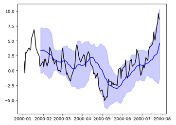
# 下面展示如何画类似bolling带的图
import pandas as pd
import matplotlib.pyplot as plt
df = pd.DataFrame({'Age': [22, 12, 18, 25, 30],
'Height': [155,129,138,164,145],
'Weight': [60,40,45,55,60]})
ax=df.plot(kind='line', x='Age', y='Height', color='DarkBlue')
ax2=df.plot(kind='line', x='Age', y='Weight', secondary_y=True,color='Red', ax=ax)
ax.set_ylabel('Height')
ax2.set_ylabel('Weight')
plt.tight_layout()
plt.show()
groupby
Change first element of each group in pandas DataFrame
df.loc[df.groupby('vintage')['val2'].head(1).index, 'val2'] = np.NaN

# groupby之后实际上就是一个一个小的dataframe,所以如果需要复杂加工可以,针对这些小的dataframe进行操作,操作完毕之后再合并,具体可以见xbx框架中处理资金曲线时对groupby的使用方式
for _index, group in df.groupby('start_time'):
  pass

# method可以是一些聚合函数也可以是lambda表达式
groupby.apply(method)

# itertools.groupy和dataframe groupby的差异只会讲相邻的group by在一起
def calc_trade_continue_perf(trade):
    """
    计算最大连续盈利和亏损
    :param trade: 订单列表,需要包含change字段表示该笔交易的net_value变化
    :return: max_continue_profit_count, max_continue_profit, max_continue_loss_count, max_continue_loss
    """
    import itertools

    continue_trx_lists = []
    max_continue_loss_count = 0
    max_continue_profit_count = 0

    # itertools.groupy和dataframe groupby的差异只会讲相邻的group by在一起
    for k, l in itertools.groupby(trade.iterrows(), key=lambda row: -1 if row[1]['change'] < 0 else 1):
        trade_change = np.array([t[1]['change'] for t in l])
        _length = len(trade_change)

        if k == -1 and _length > max_continue_loss_count:
            max_continue_loss_count = _length
        if k == 1 and _length > max_continue_profit_count:
            max_continue_profit_count = _length

        continue_change_compound = np.cumprod(1 + trade_change)[-1]
        continue_trx_lists.append(continue_change_compound)

    max_continue_loss = 1 - min(continue_trx_lists)
    max_continue_profit = max(continue_trx_lists) - 1
    return [max_continue_profit_count, max_continue_profit, max_continue_loss_count, max_continue_loss]
其他
pandas 处理缺失值dropna、drop、fillna
df = pd.DataFrame([3, 5, 6, 2, 4, 6, 7, 8, 7, 8, 9])
df.values.tolist()
将df转化成[[],[]]

#显示所有列
pd.set_option('display.max_columns', None)
#显示所有行
pd.set_option('display.max_rows', None)
#查看列数据类型
df.dtypes
#将读取的日期转为datatime格式
df['c'] = pd.to_datetime(df['c'],format='%Y-%m-%d %H:%M:%S')
#将某个datetime类型的列转化成string
btc_df['date'] = btc_df['date'].dt.strftime('%Y-%m-%d')
#新增一个列,并且根据已有的值进行赋值,机器fgi_map是某个map,根据这个进行赋值
btc_df["fgi"] = btc_df.apply(lambda x: fgi_map[x.date] if x.date in fgi_map else np.nan, axis=1)
# column 改为 index
df.set_index('date', inplace=True)
#(all)index 改为 column
df.reset_index()
#(the first)index 改为 column
df.(level=0, inplace=True)
# pandas的merge方法提供了一种类似于SQL的内存链接操作
result = pd.merge(left, right, on=['key1', 'key2'])


df = pd.DataFrame({"name": ['Alfred', 'Batman', 'Catwoman'],
   "toy": [np.nan, 'Batmobile', 'Bullwhip'],
   "born": [pd.NaT, pd.Timestamp("1940-04-25")
            pd.NaT]})

# Define in which columns to look for missing values.
>>> df.dropna(subset=['name', 'born'])
name        toy       born
1    Batman  Batmobile 1940-04-25

# 进行绘图
tsla_df[['close', 'volume']].plot(subplots=True, style=['r', 'g'], grid=True);

tsla_df[(np.abs(tsla_df.p_change) > 8) & (tsla_df.volume > 2.5 * tsla_df.volume.mean())]

format = lambda x: '%.2f' % x
tsla_df.atr21.map(format).tail()

data["gender"] = data["gender"].map({"男":1, "女":0})

# 同时Series对象还有apply方法,apply方法的作用原理和map方法类似,区别在于apply能够传入功能更为复杂的函数。
def apply_age(x,bias):
    return x+bias

#以元组的方式传入额外的参数
data["age"] = data["age"].apply(apply_age,args=(-3,))

#返回形状,即几行几列的数组,如[2,3]
shape=dataframe.shape()
rows=shape[0]
columns=shape[1]


df = pd.DataFrame({'a':[1,2,np.nan], 'b':[np.nan,np.nan,np.nan]})
# df['b'].count()可以计算b这个列非nan的数量
>>> df['b'].count()
0
>>> df['a'].count()
2

# columns可以查看列名
>>> df.columns
Index(['a', 'b'], dtype='object')
>>> df.columns[0]
'a'
import numpy as np
>>> a = np.array([1,2,3])
>>> np.cumprod(a) # intermediate results 1, 1*2
...               # total product 1*2*3 = 6
array([1, 2, 6])
>>> a = np.array([[1, 2, 3], [4, 5, 6]])
>>> np.cumprod(a, dtype=float) # specify type of output
array([   1.,    2.,    6.,   24.,  120.,  720.])


>>>
>>> np.cumprod(a, axis=0) # The cumulative product for each column (i.e., over the rows) of a:
array([[ 1,  2,  3],
       [ 4, 10, 18]])

>>>
>>> np.cumprod(a,axis=1) # The cumulative product for each row (i.e. over the columns) of a:
array([[  1,   2,   6],
       [  4,  20, 120]])


series = pd.Series([1, 5, 7, 2, 4, 6, 9, 3, 8, 10])

In [194]: series.rolling(window = 3, center = True).quantile(.5)
# shift方法,index不会移动,数据会进行移动,因此会导致最后一行直接移到空气中,可以参见下面的方式,在头部增加一行数据

# 如果第一行不一致的话,需要将原始数据的第一行补充进来,否则会导致开始日期不对,导致收益率不对
if result['candle_begin_time'].iloc[0] != df['candle_begin_time'].iloc[0]:
	result = result.append(result.iloc[-1].copy())
	result = result.shift()
	result.iloc[0] = df.iloc[0].copy()
	result['equity_change'].iloc[0] = 0
	result['equity_curve'].iloc[0] = 1